08 Sep 2022

Tiny Telematics: Tracking my truck's location offline with a Raspberry Pi, redis, Kafka, and Flink (Part 2)

Introduction

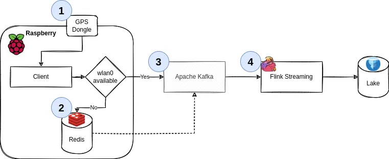
This is Part 2. Part 1 can be found here, where we discussed goals and architecture, built a custom Raspbian Linux image, implemented the client part of the application in Python, using gpsd, with concepts borrowed from scala.

Or, take it from the GitHub page:

Track your vehicle’s live location offline by using little more than a Raspberry Pi & a gps dongle (aka “Tiny Telematics”)

This time, we’ll…

We’ll do a quick architecture recap.
Then, setting up a lot of infrastructure: Flink, Kafka, mariaDB, mostly via Docker
Then, we’ll build a streaming pipeline in Flink: Fun times in scala! Additional guests: newtype, circe, and others!
Test this on the road
Use Apache Superset to visualize the data
Talk about things that broke & lessons learned
Discuss next steps

We should wind up with something like this. [Credit: Author]

All code can be found on GitHub.

Architecture Recap

Just as a reminder, what we’re doing here:

Use gpsd to get geo data from a physical USB GPS dongle
Work offline by default. Cache all your data if there’s no internet available
If you can (i.e., are online), publish all your data to a streaming pipeline via Kafka
Said pipeline persists the data

Setup up a Backend

In Part 1, we built a good execution environment in the frontend, we can do the same for the backend - i.e., the Kafka cluster and storage. This is where things go from “low level stuff” to “pretend a Docker container can abstract the complexities of distributed systems away”. I’m still very grateful for it, having set up multiple bare-metal Hadoop environments in my time. This is easier for protoyping and at-home use.

Kafka & Negotiating brokers

Since we don’t need a large, fancy cluster & the server isn’t reachable from the internet anyways (i.e., we don’t need auth), we can get away with the following on your server.

 1
 2
 3
 4
 5
 6
 7
 8
 9
10
11
12
13
# Add your user - we did this in the image earlier, but you might want this locally too
sudo useradd -m -g users -G docker telematics
sudo passwd telematics
sudo su - telematics
# Take the default docker-compose.yaml (see below)
vim docker-compose.yaml
# Start it
docker-compose up -d
# Start a topic
docker exec broker \
kafka-topics --bootstrap-server broker:9092 \
             --create \
             --topic telematics

This is also how I run Kafka locally at work (just via podman) - it’s fantastic to have on your laptop if you’re a heavy Kafka user.

For the docker-compose.yaml, see https://developer.confluent.io/quickstart/kafka-docker/

 1
 2
 3
 4
 5
 6
 7
 8
 9
10
11
12
13
14
15
16
17
18
19
20
21
22
23
24
25
26
27
28
---
version: '3'
services:
  zookeeper:
    image: confluentinc/cp-zookeeper:7.0.1
    container_name: zookeeper
    environment:
      ZOOKEEPER_CLIENT_PORT: 2181
      ZOOKEEPER_TICK_TIME: 2000

  broker:
    image: confluentinc/cp-kafka:7.0.1
    container_name: broker
    ports:
    # To learn about configuring Kafka for access across networks see
    # https://www.confluent.io/blog/kafka-client-cannot-connect-to-broker-on-aws-on-docker-etc/
      - "9092:9092"
      - "19092:19092"
    depends_on:
      - zookeeper
    environment:
      KAFKA_BROKER_ID: 1
      KAFKA_ZOOKEEPER_CONNECT: 'zookeeper:2181'
      KAFKA_LISTENER_SECURITY_PROTOCOL_MAP: PLAINTEXT:PLAINTEXT,PLAINTEXT_INTERNAL:PLAINTEXT,EXTERNAL_DIFFERENT_HOST:PLAINTEXT
      KAFKA_ADVERTISED_LISTENERS: PLAINTEXT://localhost:9092,PLAINTEXT_INTERNAL://broker:29092,EXTERNAL_DIFFERENT_HOST://bigiron.lan:19092
      KAFKA_OFFSETS_TOPIC_REPLICATION_FACTOR: 1
      KAFKA_TRANSACTION_STATE_LOG_MIN_ISR: 1
      KAFKA_TRANSACTION_STATE_LOG_REPLICATION_FACTOR: 1

Please note the inclusion of EXTERNAL_DIFFERENT_HOST to ensure the initial Kafka broker (bigiron.lan:9092) returns the correct address for the client to connect to. See here for an explanation. If you don’t see this, the next step will yield something along the lines of:

1
 WARN [Producer clientId=console-producer] Connection to node 1 (localhost/127.0.0.1:9092) could not be established. Broker may not be available. (org.apache.kafka.clients.NetworkClient)

As bigiron.lan:9092 tells us “hey, talk to localhost:9092”, which of course, isn’t the correct machine. bigiron.lan, of course, is curtesy of my DNS resolver knowing about bigiron’s IP.

Anyways, we can test this from our RasPi or laptop via:

 1
 2
 3
 4
 5
 6
 7
 8
 9
10
11
# Download & install
sudo mkdir -p /opt/kafka && cd /opt/kafka
sudo wget https://downloads.apache.org/kafka/3.2.1/kafka-3.2.1-src.tgz
sudo tar -xzf kafka-3.2.1-src.tgz
sudo ln -s /opt/kafka/kafka-3.2.1-src /opt/kafka/latest
sudo /opt/kafka/latest/gradlew jar -PscalaVersion=2.13.6

# bigiron.lan is https://chollinger.com/blog/2019/04/building-a-home-server/
/opt/kafka/latest/bin/kafka-console-producer.sh --bootstrap-server bigiron.lan:19092 \
                       --topic telematics
> test

You can do this via docker as well, I think. I just chose not to - I like my cli tools be cli tools and the services to be services (i.e., containers nowadays). I’ve run Linux servers for well over a decade and docker has been a godssent for services.

Anyhow, to make sure it works:

1
2
3
4
5
telematics@bigiron:~$ docker exec --interactive --tty broker \
kafka-console-consumer --bootstrap-server broker:9092 \
                       --topic telematics \
                       --from-beginning
test

Wonderful!

As much as I like simple docker deploys, I’m sure we can all agree that this is not the way you’d deploy this in production @ work… but the server in my basement is also not exactly a data center.

Storage & DDL

Originally, I wanted to use Apache Iceberg for this part, but we’ll stick to a standard MariaDB instance for now. You can grab a copy here.

Our table definition looks like this:

 1
 2
 3
 4
 5
 6
 7
 8
 9
10
11
12
13
CREATE TABLE telematics.trips (
    `id` BIGINT NOT NULL AUTO_INCREMENT,
	`tripId` BIGINT NOT NULL,
	`userId` BIGINT NOT NULL,
     -- DOUBLE in MySql lacks the precision for geospatial data!
	`lat` DECIMAL(11,8),
	`lon` DECIMAL(11,8),
	`altitude` DOUBLE,
	`speed` DOUBLE,
	`ts` TIMESTAMP NOT NULL,
	`updated_at` TIMESTAMP NOT NULL,
	PRIMARY KEY(id)
);

Which is simply the model translated into sql.

Types!

Note the type for lat and lon as DECIMAL. Most people are familiar with very strict types in sql, but somehow not in e.g. Python. We’ll get back to that momentarily. For this example, consider the following:

34.42127702575059, -84.11905647651372 is Downtown Dawsonville, GA. (34.4, -84.1) is 2.2 miles away, (34.0, -84.0) is 40 miles away in Lawrenceville, GA. That’s DECIMAL(11,8) vs DOUBLE vs FLOAT in MariaDB (the latter, more or less, but it drives home a point).

Keep in mind:

decimal places	degrees	distance
0	1.0	111 km
1	0.1	11.1 km
2	0.01	1.11 km
3	0.001	111 m
4	0.0001	11.1 m
5	0.00001	1.11 m
6	0.000001	0.111 m
7	0.0000001	1.11 cm
8	0.00000001	1.11 mm

Source: http://wiki.gis.com/wiki/index.php/Decimal_degrees

I know most people are familiar - but it is worth pointing out early in the process.

Building a Streaming Pipeline

While Part 1 talked a lot about low-tech and nitty-gritty details, we’re now moving from low to high-tech: Let’s talk streaming. Briefly.

About Apache Flink

Now, we have infrastructure, we have a producer application (with a cache!), let’s talk about consuming these events. We’ll use Apache Flink:

If you used something like Spark, Storm, Heron, or Beam before, this is nothing new conceptually. Since I don’t have the space or time to talk about when you’d use what, let’s just leave it at this: Stateful, real-time stream processing with either bounded or unbounded streams and several layers of abstraction that allow you to write both very simple, boilerplated jobs, as well as complex stream processing pipelines that can do really cool stuff.

What makes Flink interesting for this project in particular (besides the fact that I want to play around with it) is twofold:

If we ever wanted to graduate from MariaDB, Flink has an Apache Iceberg connector, as well as a JDBC connector, which makes writing data much easier than having to roll our own.

Secondly, the way it approaches snapshots: While I invite you to read the linked tech doc, a (rough) two sentence summary is:

A barrier separates the records in the data stream into the set of records that goes into the current snapshot, and the records that go into the next snapshot. […]
Once the last stream has received barrier n, the operator emits all pending outgoing records, and then emits snapshot n barriers itself.

This means, we can process with exactly-once semantics; remember that our producer guarantees are “at least once”, so the best stateful snapshotting process in the world won’t save us from producing duplicates if we introduce them ourselves. [1]

However, unless latency is a top priority (which here, it clearly isn’t, as we’re already caching most of our data and have at most a handful of users, one for each vehicle in the household), adding a handful of ms of latency to our stream for the benefit of getting exactly-once semantics will greatly increase the resulting data quality.

Also, Flink has a neat, persistent UI, which e.g. Spark still really doesn’t have.

Note: We need scala 2.12.16, not 2.13.x:

1
2
sdk use scala 2.12.16
sbt compile

[1] You’ll quickly note that, while possible (and I called out how to do it), the pipeline presented herein isn’t actually following exactly-once semantics yet. I plan to add that in the future after I replace MariaDB - currently, the abstraction from a full database to a decoupled storage and compute engine is too weak to spend the effort in making this exactly-once, since I’d have to do it again later on.

Getting started

We can start by getting the sbt quickstart set up:

1
bash <(curl https://flink.apache.org/q/sbt-quickstart.sh)

This generates an template project we can customize.

The job we need is deceptively simple:

Read from Kafka in an unbounded stream; make sure the messages are keyed by client
Write them to a sink, e.g. Iceberg files or a JDBC sink, periodically & snapshot after

Standard Flink vs. Libraries

I’m adding a handful of, in my opinion, good-practice scala libraries to Flink, which is not something you’ll see in many tutorials for Flink or any Data Engineering articles. Most of them are inspired by Gabriel Volpe’s excellent “Practical FP in Scala” book.

The Domain Model

First things first: Let’s make sure we have our domain model ready to go. The heavy lifting was done beforehand, so this should be easy.

Modeling

We’ll make full use of a smart type system and model our @dataclass from Python in scala as unambiguous as possible:

 1
 2
 3
 4
 5
 6
 7
 8
 9
10
11
12
13
14
class GpsModel {

  sealed trait GpsMeasurement{
    def value: Double
  }
  final case class Latitude(value: Double) extends GpsMeasurement
  final case class Longitude(value: Double) extends GpsMeasurement

  @newtype final case class Altitude(meters: Double)
  @newtype final case class Speed(metersPerSecond: Double)

  type ID = Long
  final case class GpsPoint(tripId: ID, userId: ID, lat: Latitude, lon: Longitude, altitude: Altitude, speed: Speed, timestamp: EpochMs)
}

Note that this time we’ll always have real 64bit values available.

We’ll rely on the ever-useful newtype library, as well as circe for JSON SerDe (see below).

Keep in mind, since we have to use scala 2.12, we need to add

1
addCompilerPlugin("org.scalamacros" % "paradise" % "2.1.1" cross CrossVersion.full)

to the build.sbt.

Serializing & Deserializing: JSON

Since we probably don’t want to write our own SerDe by hand, we can use derevo to automatically derive encoders and decoders by using some compiler annotations:

 1
 2
 3
 4
 5
 6
 7
 8
 9
10
  @derive(encoder, decoder)
  final case class GpsPoint(
      tripId: ID,
      userId: ID,
      lat: Latitude,
      lon: Longitude,
      altitude: Altitude,
      speed: Speed,
      timestamp: EpochMs
  )

Which is neat, because now, we can get import io.circe.syntax.EncoderOps into scope and say:

1
2
3
val p = GpsPoint( // ...)
p.asJson
// {"userId":85383823942605,"lat":10.0,"lon":-10.0,"altitude":0.0,"speed":0.0,"timestamp":1660690181680}

We can easily test this for isomorphism by writing a unit test:

 1
 2
 3
 4
 5
 6
 7
 8
 9
10
11
12
13
14
15
16
17
18
19
20
class GpsModelTest extends AnyFunSuite {
  test("GpsPoint encodes both ways") {
    val p = GpsPoint(
      100L,
      0x4da7f87ee3cdL,
      Latitude(10.0),
      Longitude(-10.0),
      Altitude(0.0),
      Speed(0.0),
      1660690181680L
    )
    val json: Json = p.asJson
    val decoded    = jawn.decode[GpsModel.GpsPoint](json.noSpaces)
    assert(decoded.isRight)
    decoded match {
      case Right(p2) => assert(p2 == p)
      case _         => assert(false)
    }
  }
}

However, when dealing with newtypes, we sometimes might need to write our own encoders and decoders:

 1
 2
 3
 4
 5
 6
 7
 8
 9
10
11
12
13
14
15
  @newtype final case class Altitude(meters: Double)
  object Altitude {
    implicit val encoder: Encoder[Altitude] = new Encoder[Altitude]() {
      override def apply(a: Altitude): Json = a.meters.asJson
    }
    implicit val decoder: Decoder[Altitude] = new Decoder[Altitude]() {
      override def apply(c: HCursor): Result[Altitude] = {
        for {
          v <- c.value.as[Double]
        } yield {
          new Altitude(v)
        }
      }
    }
  }

Which, while possible, is mildly awkward; by default, it would encode it as:

1
{"userId":85383823942605,"lat":{"value":10.0},"lon":{"value":-10.0},"altitude":0.0,"speed":0.0,"timestamp":1660690181680}

Note the "value: 10.0" map, rather than having a straight mapping as "lat": 10.0. [1]

Since we probably won’t need custom apply() and unapply() methods or other shenanigans, this led me to simplify our model to:

 1
 2
 3
 4
 5
 6
 7
 8
 9
10
11
12
13
14
15
16
17
18
19
20
  type Meters          = Double
  type MetersPerSecond = Meters
  type Latitude        = Meters
  type Longitude       = Meters
  type Altitude        = Meters
  type Speed           = MetersPerSecond

  type ID = String
  @derive(encoder, decoder)
  final case class GpsPoint(
      id: ID,
      lat: Latitude,
      lon: Longitude,
      altitude: Altitude,
      speed: Speed,
      timestamp: Long
  )
  object GpsPoint {
    implicit val typeInfo: TypeInformation[GpsPoint] = TypeInformation.of(classOf[GpsPoint])
  }

[1] If there’s an easier way around that, somebody please let me know.

Reading from Kafka

Now, going from and to string is cool, but not quite what we need when we need to talk to Kafka. Take a look at the following function:

 1
 2
 3
 4
 5
 6
 7
 8
 9
10
11
12
13
14
15
16
17
18
19
20
21
22
23
24
25
26
27
28
29
30
31
32
33
34
35
36
  def buildSource[A](
      bootstrapServers: String,
      topics: String,
      groupId: String
  )(implicit
      deserializer: Decoder[A],
      typeInfo: TypeInformation[A]
  ): KafkaSource[A] = {
    KafkaSource
      .builder[A]
      .setBootstrapServers(bootstrapServers)
      .setTopics(topics)
      .setGroupId(groupId)
      // Start from committed offset, also use EARLIEST as reset strategy if committed offset doesn't exist
      .setStartingOffsets(
        OffsetsInitializer.committedOffsets(OffsetResetStrategy.EARLIEST)
      )
      .setDeserializer(
        new KafkaRecordDeserializationSchema[A] {
          override def deserialize(
              record: ConsumerRecord[Array[Byte], Array[Byte]],
              out: Collector[A]
          ): Unit = {
            val s                         = new StringDeserializer().deserialize(topics, record.value())
            val v: Either[circe.Error, A] = jawn.decode[A](s)
            v match {
              case Left(e)      => println(e)
              case Right(value) => out.collect(value)
            }
          }

          override def getProducedType: TypeInformation[A] = typeInfo
        }
      )
      .build
  }

Now this looks a little more complicated that it needs to, so let’s break it down.

Signature & Types

The signature is A => KafkaSource[A], with KafkaSource being a

1
2
3
public class KafkaSource<OUT>
        implements Source<OUT, KafkaPartitionSplit, KafkaSourceEnumState>,
                ResultTypeQueryable<OUT> 

The type of the function is A without any bounds (if you’re suspicious, carry on).

The arguments ask for three Strings, which could new @newtype’d if you want to, and all three simply refer to standard Kafka settings we’ve already discussed. We’ll refactor this in a minute once we load a config file.

1
2
3
4
5
6
7
8
 def buildSource[A](
      bootstrapServers: String,
      topics: String,
      groupId: String
  )(implicit
      deserializer: Decoder[A],
      typeInfo: TypeInformation[A]
  ): KafkaSource[A] = 

The last section asks for 2 implicits: A Decoder[A] and TypeInformation[A]. These are, essentially type bounds that say “the type A must have a Decoder and TypeInformation available and in scope”.

A Decoder can be provided by derevo, see above. TypeInformation can be inferred as such:

1
2
3
  object GpsPoint {
    implicit val typeInfo: TypeInformation[GpsPoint] = TypeInformation.of(classOf[GpsPoint])
  }

This means, we can also express this by means of a type class:

1
def buildSource[A: Decoder : TypeInformation]

Which would be simply sugar for the aforementioned implicits. As long as we have everything in scope, we simply define very clear bounds for the type of A, meaning if you don’t tell it how to deserialize your weird custom data structures, it won’t to it.

Building a source

The next part simply sets up our FlinkSource. The only thing of note is the comment above setStartingOffset:

1
2
3
4
5
6
7
8
9
    KafkaSource
      .builder[A]
      .setBootstrapServers(bootstrapServers)
      .setTopics(topics)
      .setGroupId(groupId)
      // Start from committed offset, also use EARLIEST as reset strategy if committed offset doesn't exist
      .setStartingOffsets(
        OffsetsInitializer.committedOffsets(OffsetResetStrategy.EARLIEST)
      )

Deserializing

Unsurprisingly, we’ll now use the aforementioned implicit Decoder[A] to build a concrete instance of a KafkaRecordDeserializationSchema by taking the incoming, raw Array[Byte] from Kafka and piping them through circe back to JSON back to a scala object:

 1
 2
 3
 4
 5
 6
 7
 8
 9
10
11
12
13
14
15
16
17
      .setDeserializer(
        new KafkaRecordDeserializationSchema[A] {
          override def deserialize(
              record: ConsumerRecord[Array[Byte], Array[Byte]],
              out: Collector[A]
          ): Unit = {
            val s                         = new StringDeserializer().deserialize(topics, record.value())
            val v: Either[circe.Error, A] = jawn.decode[A](s)
            v match {
              case Left(e)      => println(e)
              case Right(value) => out.collect(value)
            }
          }

          override def getProducedType: TypeInformation[A] = typeInfo
        }
      )

And that’s our source!

Writing to the database

This can be done via the standard JDBC connector. Keep in mind that in order to support exactly-once delivery, your database needs to support the XA Spec.

That being said, all we need to do in the Flink world is convert some Java to scala syntax.

 1
 2
 3
 4
 5
 6
 7
 8
 9
10
11
12
13
14
15
16
17
18
  def jdbcSink(config: JdbcConfig): SinkFunction[GpsPoint] = {
    JdbcSink.sink[GpsPoint](
      GpsPoint.query,
      GpsPoint.statement,
      JdbcExecutionOptions
        .builder()
        .withBatchSize(1000)
        .withBatchIntervalMs(200)
        .withMaxRetries(5)
        .build(),
      new JdbcConnectionOptions.JdbcConnectionOptionsBuilder()
        .withUrl(config.url)
        .withDriverName(config.driverName)
        .withUsername(config.user)
        .withPassword(config.password)
        .build()
    )
  }

But our statement builder has to be very Java-esque and mutable:

 1
 2
 3
 4
 5
 6
 7
 8
 9
10
11
12
13
14
15
16
17
18
19
20
21
  object GpsPoint {
    implicit val typeInfo: TypeInformation[GpsPoint] = TypeInformation.of(classOf[GpsPoint])
    val query: String =
      "insert into trips (tripId, userId, lat, lon, altitude, speed, ts, updated_at) values (?, ?, ?, ?, ?, ?, ?, ? )"
    // noinspection ConvertExpressionToSAM
    // Otherwise: Caused by: java.io.NotSerializableException: Non-serializable lambda
    def statement: JdbcStatementBuilder[GpsPoint] = {
      new JdbcStatementBuilder[GpsPoint] {
        override def accept(statement: PreparedStatement, e: GpsPoint): Unit = {
          statement.setLong(1, e.tripId)
          statement.setLong(2, e.userId)
          statement.setDouble(3, e.lat) // <- Double is fine here, it has enough precision in scala!
          statement.setDouble(4, e.lon)
          statement.setDouble(5, e.altitude)
          statement.setDouble(6, e.speed)
          statement.setTimestamp(7, new Timestamp(e.timestamp))
          statement.setTimestamp(8, new Timestamp(new Date().getTime))
        }
      }
    }
  }

Configuration

You’ve seen it in the previous section, but we’ll use pureconfig for reading config files. To keep it simple, we’ll define a minimal model and read it from resources/application.conf:

 1
 2
 3
 4
 5
 6
 7
 8
 9
10
object Config {
  final case class Config(kafka: KafkaConfig, jdbc: JdbcConfig)
  final case class KafkaConfig(bootstrapServers: String, topics: String, groupId: String)
  final case class JdbcConfig(url: String, driverName: String, user: String, password: String)

  def loadConfig(): Either[ConfigReaderFailures, Config] = sys.env.get("RUN_LOCALLY") match {
    case Some(_) => ConfigSource.default.load[Config]
    case _       => ConfigSource.resources("production.conf").load[Config]
  }
}

Putting it all together

Lastly, we’ll need an entrypoint:

 1
 2
 3
 4
 5
 6
 7
 8
 9
10
11
12
13
14
15
16
17
18
19
20
21
22
23
24
25
26
27
28
  def main(args: Array[String]): Unit = {
    // Require a streaming environment
    val env = StreamExecutionEnvironment.getExecutionEnvironment
    env.setRestartStrategy(
      RestartStrategies.fixedDelayRestart(
        3,                            // number of restart attempts
        Time.of(10, TimeUnit.SECONDS) // delay
      )
    )
    // Load config
    val config = Config.loadConfig() match {
      case Right(c) => c
      case Left(e)  => throw new Exception(e.prettyPrint())
    }
    // Build source
    implicit val encoder: Encoder[GpsPoint] = implicitly
    val data: DataStream[GpsPoint] = env.fromSource(
      buildSource[GpsPoint](config.kafka),
      WatermarkStrategy.forBoundedOutOfOrderness(JDuration.ofSeconds(10)),
      "Kafka Source"
    )
    // Print for testing
    val _: DataStreamSink[GpsPoint] = data.print()
    // Write to JDBC
    data.addSink(Sinks.jdbcSink(config.jdbc))
    // execute program
    env.execute("Telematics v3")
  }

To test our job, we can run sbt run and it’ll consume previously collected data from Kafka:

1
[info] 11> GpsPoint(61573282483598,0.0,0.0,0.0,0.0,1659355200000)

And writes it diligently to MariaDB:

Cluster Setup

We’ll run this on a simple, single-node cluster in session mode, which allows us to submit jobs towards the cluster. Once again, we can containerize all this:

 1
 2
 3
 4
 5
 6
 7
 8
 9
10
11
12
13
14
15
16
17
18
19
20
21
22
23
version: "2.2"
services:
  jobmanager:
    image: flink:latest
    ports:
      - "8082:8081"
    command: jobmanager
    environment:
      - |
        FLINK_PROPERTIES=
        jobmanager.rpc.address: jobmanager                

  taskmanager:
    image: flink:latest
    depends_on:
      - jobmanager
    command: taskmanager
    scale: 1
    environment:
      - |
        FLINK_PROPERTIES=
        jobmanager.rpc.address: jobmanager
        taskmanager.numberOfTaskSlots: 2               

And we can submit the job:

1
2
3
4
5
sbt clean assembly
flink run \
      --detached \
      --jobmanager bigiron.lan:8082 \
      ./target/scala-2.12/TinyTelematics-assembly-0.1.jar

Road Test

Time to take this on the road and see what happens.

Infrastructure Launch Check

Now that we have all components ready to go, let’s go over the infrastructure one more time:

Kafka

Kafka runs in docker on a remote server that’s accessible on the local subnets.

Flink

Flink runs in session mode and executes our job from before.

MariaDB

The database is not something we’ve set up in this article, but has been running diligently forever.

Raspberry Pi

The Raspberry Pi runs our client app :

 1
 2
 3
 4
 5
 6
 7
 8
 9
10
11
12
telematics@raspberrypi:/var/log/telematics$ sudo service tiny-telematics status
● tiny-telematics.service - tiny-telematics
     Loaded: loaded (/etc/systemd/system/tiny-telematics.service; enabled; vendor preset: enabled)
     Active: active (running) since Sun 2022-08-01 00:00:00 EDT; 32s ago
   Main PID: 3877 (run_client.sh)
      Tasks: 4 (limit: 415)
        CPU: 31.240s
     CGroup: /system.slice/tiny-telematics.service
             ├─3877 /bin/bash /home/telematics/TinyTelematics/sbin/run_client.sh
             ├─4029 /bin/bash /home/telematics/TinyTelematics/sbin/run_client.sh
             ├─4030 /home/telematics/.pyenv/versions/3.8.13/bin/python3.8 /home/telematics/.pyenv/versions/3.8.13/bin/pip3 list
             └─4031 grep tiny-telematics

And of course, we need to confirm it survives a restart -

1
2
3
4
5
sudo reboot 0
ssh pi@pi-telematics.lan
tail -100 /var/log/telematics/err.log
# 2022-08-01 00:00:00,498 - WARNING main.py:poll_gps():94 - Empty record, filtering
# 2022-08-01 00:00:00,503 - DEBUG main.py:main():237 - No GPS record returned

Setting up the physical hardware

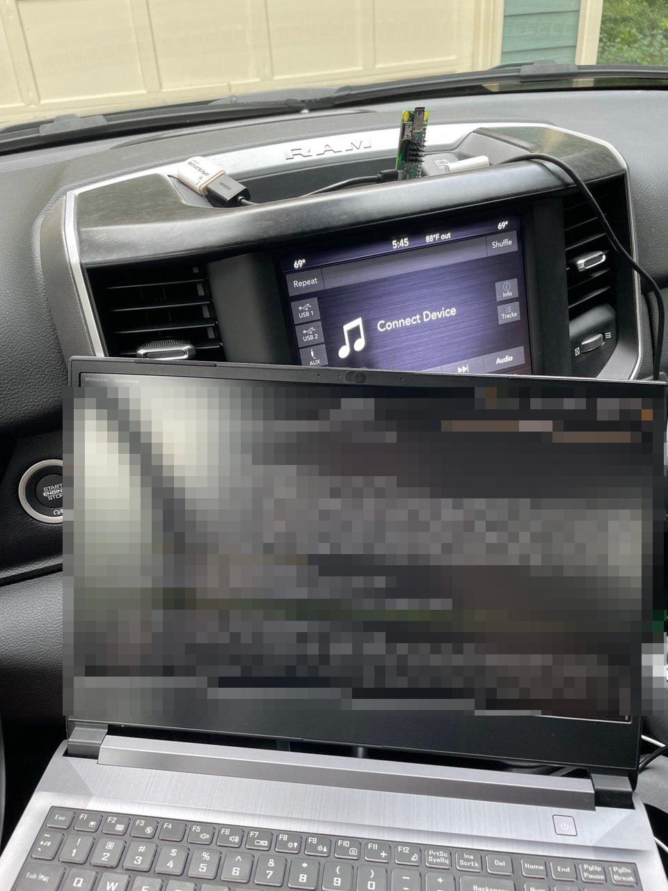
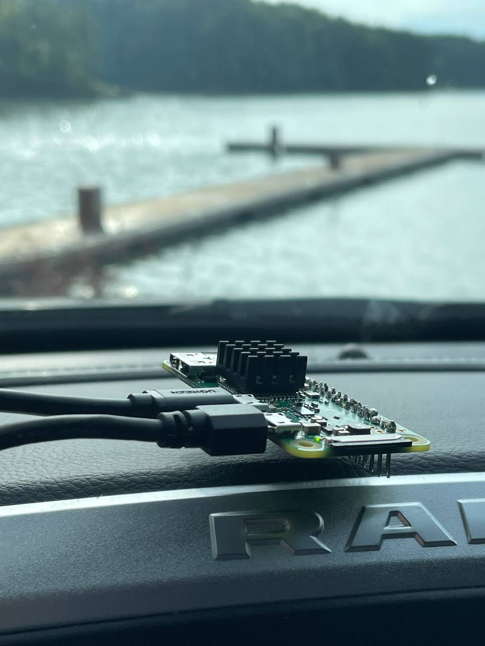
This was a matter of plugging in the Pi into a USB port and checking that everything worked:

The only mishap here was the fact that we didn’t set up any udev rules that would ensure we can always talk to e.g. /dev/ttyGps, rather than /dev/ttyACM$N, where $N might not always be consistent, resulting in a pack on GPS connectivity.

udev is a userspace system that enables the operating system administrator to register userspace handlers for events. The events received by udev’s daemon are mainly generated by the (Linux) kernel in response to physical events relating to peripheral devices. As such, udev’s main purpose is to act upon peripheral detection and hot-plugging, including actions that return control to the kernel, e.g., loading kernel modules or device firmware.
https://wiki.archlinux.org/title/udev

This can, in theory, be fixed as such:

 1
 2
 3
 4
 5
 6
 7
 8
 9
10
11
12
13
14
15
16
pi@raspberrypi:~ $ udevadm info /dev/ttyACM0
P: /devices/platform/soc/20980000.usb/usb1/1-1/1-1:1.0/tty/ttyACM0
N: ttyACM0
L: 0
S: gps0
S: serial/by-id/usb-u-blox_AG_-_www.u-blox.com_u-blox_7_-_GPS_GNSS_Receiver-if00
S: serial/by-path/platform-20980000.usb-usb-0:1:1.0
E: DEVPATH=/devices/platform/soc/20980000.usb/usb1/1-1/1-1:1.0/tty/ttyACM0
E: DEVNAME=/dev/ttyACM0
E: MAJOR=166
E: MINOR=0
E: SUBSYSTEM=tty
# ...

echo 'SUBSYSTEM=="tty", ATTRS{idVendor}=="1546", ATTRS{idProduct}=="01a7, SYMLINK+="ttyGPS"' >> /etc/udev/rules.d/99-com.rules
sudo udevadm control --reload

I have, however, not gotten it to work as of time of writing this. The hotfix might be stupid, but works:

 1
 2
 3
 4
 5
 6
 7
 8
 9
10
11
12
13
14
function replaceDevices(){
	for i in $(seq 0 2); do
		local id=$i
		echo "Probing /dev/ttyACM$id"
		if [[ -n $(udevadm info "/dev/ttyACM$id" | grep GPS) ]]; then 
			echo "Replacing gpsd devices with /dev/ttyACM$id"
			sed -i "s#DEVICES=\"\"#DEVICES=\"/dev/ttyACM$id\"#g" ${GPSD}
			sed -iE "s#/dev/ttyACM[0-9]#/dev/ttyACM$id#g" ${GPSD}
			echo "New gpsd config:"
			cat ${GPSD}
			break
		fi
	done
}

So is it really stupid? (yes, yes it is)

Driving around

This was distinctly one of the weirder developer environments I’ve worked in - during my test trip(s) (one graciously done by my significant other), having a Raspberry Pi and an obnoxiously blinking GPS dongle in the middle console is odd to say the least. Then again, probably less irritating than Carplay and others, so there’s that.

As seen in the TV show...? [Credit: Author]

Also, I’ll buy whoever recognizes this location a beer at the next conference. It is, unfortunately, not our back yard.

Checking the data

Once home, the first check is to see if we have data in Kafka.

Success!

And next, in MariaDB:

1
2
SELECT COUNT(*) FROM telematics.trips WHERE lat != 0;
-- 1,798

Also a success!

Minor issues during testing

I’ll admit it - the drive to the lakes wasn’t the only test I’d have to do. There were some other issues encountered during these road tests, and I’ll sum them up briefly:

Due to the nature of the caching mechanism, it takes quite a while to the data to be sent back to Kafka. This means, if you unplug the Pi and plug it back in inside, chances are, it won’t get a GPS fix; this means the buffer doesn’t fill and hence, our data is stuck in redis. The fix is trivial - if there’s data in redis, send that after a restart.
In a similar vein, not getting a GPS fix can cause the poll_gps() loop to practically deadlock. We can time out that process, but it makes little difference, because…
…I made a fundamental error by using time.sleep() within the loop. Rather, we should be relying on the GPS receiver’s update frequency - 1Hz - because otherwise we’ll get the same record from the buffer over and over again. We need to correct drift. See below.
However, sometimes a cheap USB GPS dongle simply doesn’t get a good signal and hence, does not report GPS data or, worse, somehow does a cold boot and needs a new satellite discovery process & fix. This happened several times, where I see the first GPS point 5 to 10 minutes after I leave the house. And while where we live has been described as “chicken country” to me, in reality, it isn’t what I’d call remote - certainly not some odd GPS blind spot where it’s impossible to get enough satellites for a signal.
The Kafka client was created prematurely and assumed WiFI connection was a given, meaning the service couldn’t start up again after a stop at Costco outside WiFi range.
An indentation error & lack of unit test (despite pretty good coverage) caused the cache to be deleted prematurely.
Lastly, another fundamental hardware issue; Postmortem can be found here.

Turns out, writing a fully cached, offline system isn’t as easy as I thought.

Drift: Do not fall asleep

What we did originally: yield, do a bunch of expensive operations, time.sleep(1), go back to gpsd and ask for the next record.

However, that next record comes in at a frequency of 1-10Hz, and our other operations (especially calling subprocess can be relatively slow). So, if we encounter drift, i.e. where we’re falling behind with processing records, we have to skip them - otherwise, we’ll never catch up.

1
2
3
4
5
6
7
8
# Account for drift, i.e. the rest of the program lags behind the gpsd buffer
# In that case, just throw away records until we're current
gps_time = ts.timestamp()
now = time.time()
drift_s = now - gps_time
if drift_s >= max_drift_s:
    logger.warning("Correcting %ss drift, skipping record", drift_s)
    continue

In a similar vein: Do not yield None - that causes expensive stuff to be run without rhyme or reason.

Originally, I thought this bug alone caused this:

1
2
3
4
SELECT COUNT(*) as C, lat, lon FROM telematics.trips GROUP BY  lat, lon HAVING lat != 0;
-- 1276	33.x2	-84.x5
-- 6630	33.x0	-84.4x0
-- 2 more rows from 2 1hr each trips. x => redaction

It did not.

We’re still not moving

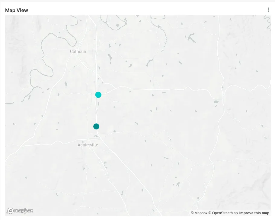
While the above rings true and was an issue, after fixing this and driving a solid 200mi one Saturday, my GPS map looked like this: [1]

The distance between those points is only a handful of miles, but I’m cropping out the rest for privacy reasons. On the real map, there’s 6 or so more points - one for each stop or restart.

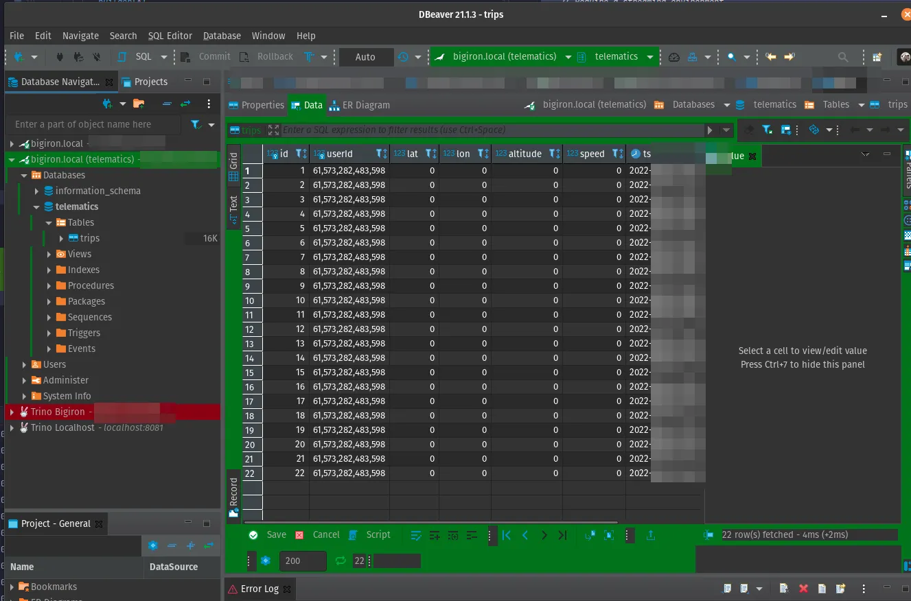
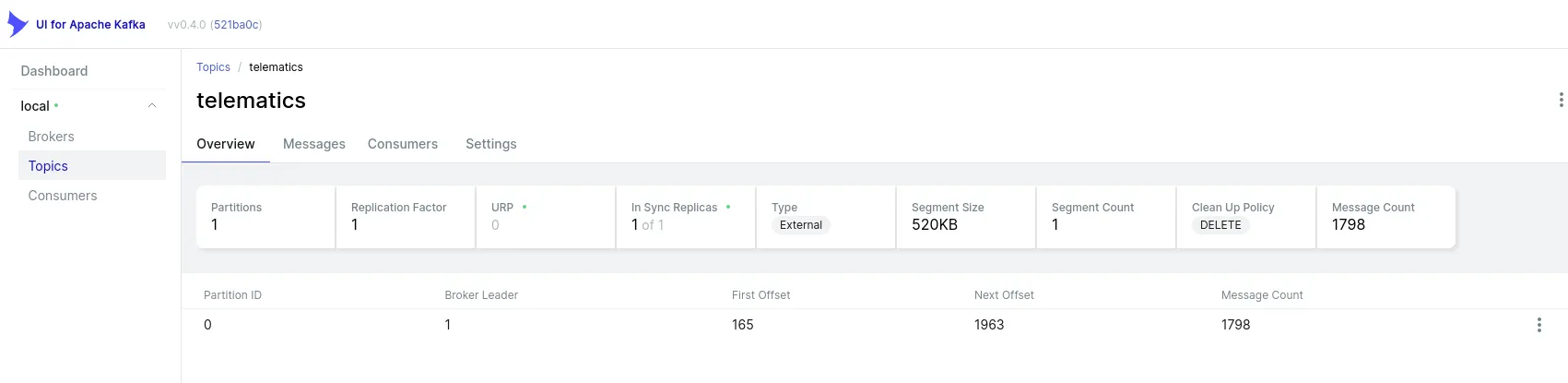
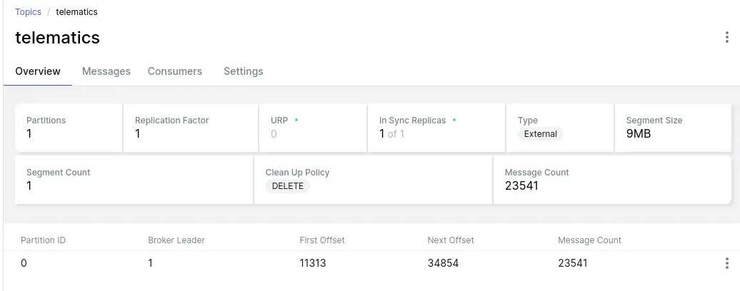
Point being: There should be hundreds of points! Matter of fact, there should be 23,541 points:

However, in sql, let’s ask for “how many points have the exact same location?”:

 1
 2
 3
 4
 5
 6
 7
 8
 9
10
SELECT COUNT(*) as C FROM telematics.trips GROUP BY  lat, lon HAVING lat != 0
ORDER BY C DESC 
-- 6028
-- 5192
-- 2640
-- 2200
-- 1885
-- 1356
-- 1320
-- ...

This is the same as before, but worse!

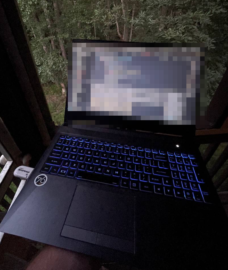
Here’s me walking around the property, staring at debug logs (our neighbors, strangely, still like us…), trying to figure out why on earth the GPS location isn’t changing - as we’ve established before, GPS isn’t super precise, but does go down to 1.11 mm in precision in theory; ergo, walking a couple of feet ought to change my location in the logs, even if only by margin of error, right?

I’ve tried everything - simulated gps data (various formats!), Python 2 style (call next()), Python 3 style (use __next__, i.e. for report in gps_client), printed out the raw (very mutable GpsClient):

 1
 2
 3
 4
 5
 6
 7
 8
 9
10
2022-08-01 00:00:00,0 - ERROR main.py:poll_gps():67 - gps_session: Time:     2022-08-01T00:00:00.000Z
Lat/Lon:  XX YY # <- real location, but always the same 
Altitude: 328.110000
Speed:    0.000000
Track:    0.000000
Status:   STATUS_NO_FIX
Mode:     MODE_3D
Quality:  4 p=9.41 h=7.40 v=5.81 t=3.49 g=10.03
Y: 18 satellites in view:
    PRN:   1  E:  19  Az: 275  Ss:   0 #....

Which changes data like satellites every time, but not the location.

Ignore the STATUS_NO_FIX - that’s frequently not reported by the receiver. MODE_3D and 17 satellites in view means it clearly can talk to the mighty sky orbs it so desperately desires.

Re-Configuring the GPS chipset

Turns out: The device I’m using, a u-blox G7020-KT (based on a u-blox 7 chip), so we can use ubxtool to get to the nitty-gritty details:

1
2
3
4
5
6
7
export UBXOPTS="-P 14"
ubxtool -p MON-VER
#UBX-MON-VER:
#  swVersion 1.00 (59842)
#  hwVersion 00070000
#  extension PROTVER 14.00
#  extension GPS;SBAS;GLO;QZSS

This means, we can fine-tune the receiver config. As the physical dongle caches configurations, including previous satellite locks and supported satellite constellations, we can simply reset the entire thing back to default:

 1
 2
 3
 4
 5
 6
 7
 8
 9
10
11
12
13
14
# This is important, but depends on your device, see PROTVER above
export UBXOPTS="-P 14"
# Reset configuration to defaults (UBX-CFG-CFG).
ubxtool -p RESET

# Disable sending of the basic binary messages.
ubxtool -d BINARY
# Enabke sending basic NMEA messages. The messages are GBS, GGA, GSA, GGL, GST, GSV, RMC, VTG, and ZDA.
# My reciever can only do basic NMEA0183 
ubxtool -e NMEA
# Enable GPS
ubxtool -e GPS
# Save
ubxtool SAVE

We can then check if everything is in-line with what we expect. The receiver I’m using is fairly primitive (only supports the L1 GPS band and uses a pretty ancient chip), but it can to up to 10Hz (allegedly), but we want the 1Hz default, so it’s a good quick check:

1
2
3
4
# Poll rate
pi ubxtool -p CFG-RATE
#UBX-CFG-RATE:
# measRate 1000 navRate 1 timeRef 1 (GPS)

Somehow, somewhere, something changed some physical aspect of my one and only GPS receiver, and that messed up all physical road tests.

Don’t believe me? Real “trip”:

Needless to say, after wasting hours of my life on this - unpaid, of course, because clearly I’m slowly loosing it - it finally worked again.

So… test your hardware, folks. And test the software running your hardware with your actual hardware, do not rely on integration tests.

This is not something I do on the daily. My hardware is in “the cloud” and consists of some Kubernetes nodes somewhere in $BIG_TECH’s datacenters.

I’ve had to debug Kernel problems, network issues, DNS issues, saw UDP used where TCP should have been used, NTP issues, crypto key exchange issues - I’m saying, I’m used to debugging stuff that’s outside of “just debug your code” (I’m sure you’re familiar).

My hardware broken, that happened once and I wrote about it. But a USB dongle (essentially a dumb terminal) being somehow mis-configured, that’s a first for me. You may laugh at me.

[1] Yes, those coordinates represent the Buc-cee’s in Calhoun, GA, and it’s wonderful.

Visualize Data

With all those issues fixed, let’s take a visual look at the data, using some fantastic open source software.

A note on the data shown

Most GPS points here are either synthetic (thanks to nmeagen.org) or altered as to avoid detailing actual trips for the purpose of this blog article (for obvious privacy reasons). In other words, I probably did not drive straight through some poor guy’s yard in Arlington, GA.

You can find a sample trip here. I’ve converted it to csv and nmea here and here which ran gpsbabel -w -r -t -i gpx -f "GraphHopper.gpx" -o nmea -F "GraphHopper.nmea". I then piped this data to the TinyTelematics application via gpsfake - everything else was running the real pipeline.

Keep in mind that this data is missing some important attributes, namely speed, altitude, and real, realistic timestamps that would drive many KPIs.

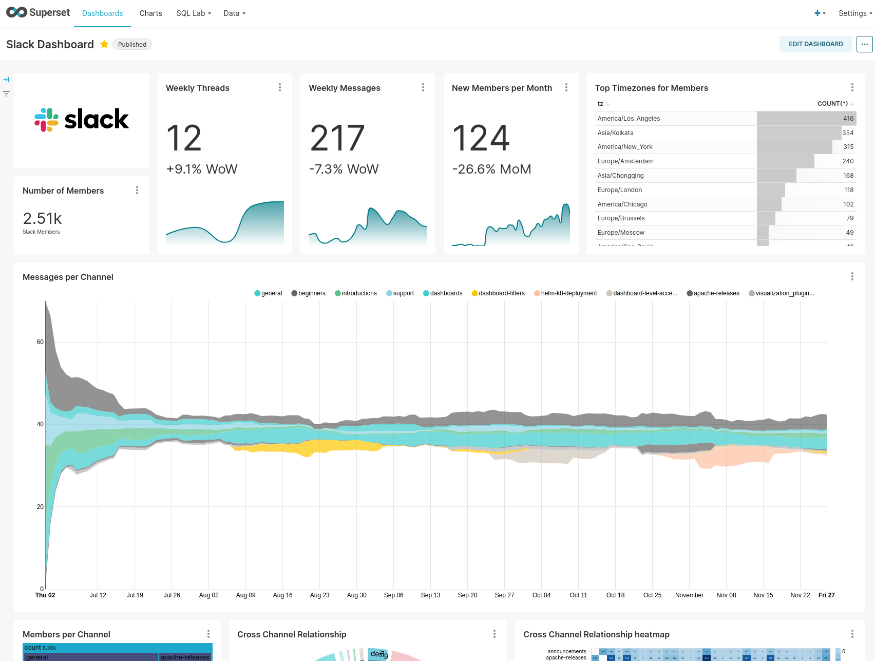
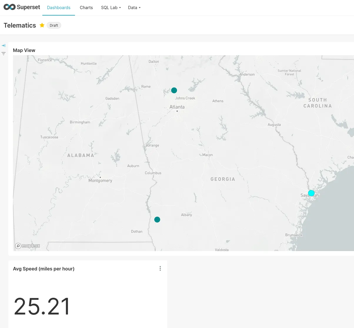
Some trips and screenshots are real.

Apache Superset

We can use Apache Superset for this. Superset is super cool - it’s a web-based, open source data visualization platform that supports MapBox for geospatial data, who have a very generous free tier.

A Superset Sample Dashboard. [Credit: Author]

We can set it up via Docker:

1
2
3
git clone https://github.com/apache/superset.git
docker-compose -f docker-compose-non-dev.yml pull
docker-compose -f docker-compose-non-dev.yml up

Note that for using mapbox, you’ll need to edit docker/.env-non-dev and add your MAPBOX_API_KEY.

Add a dataset

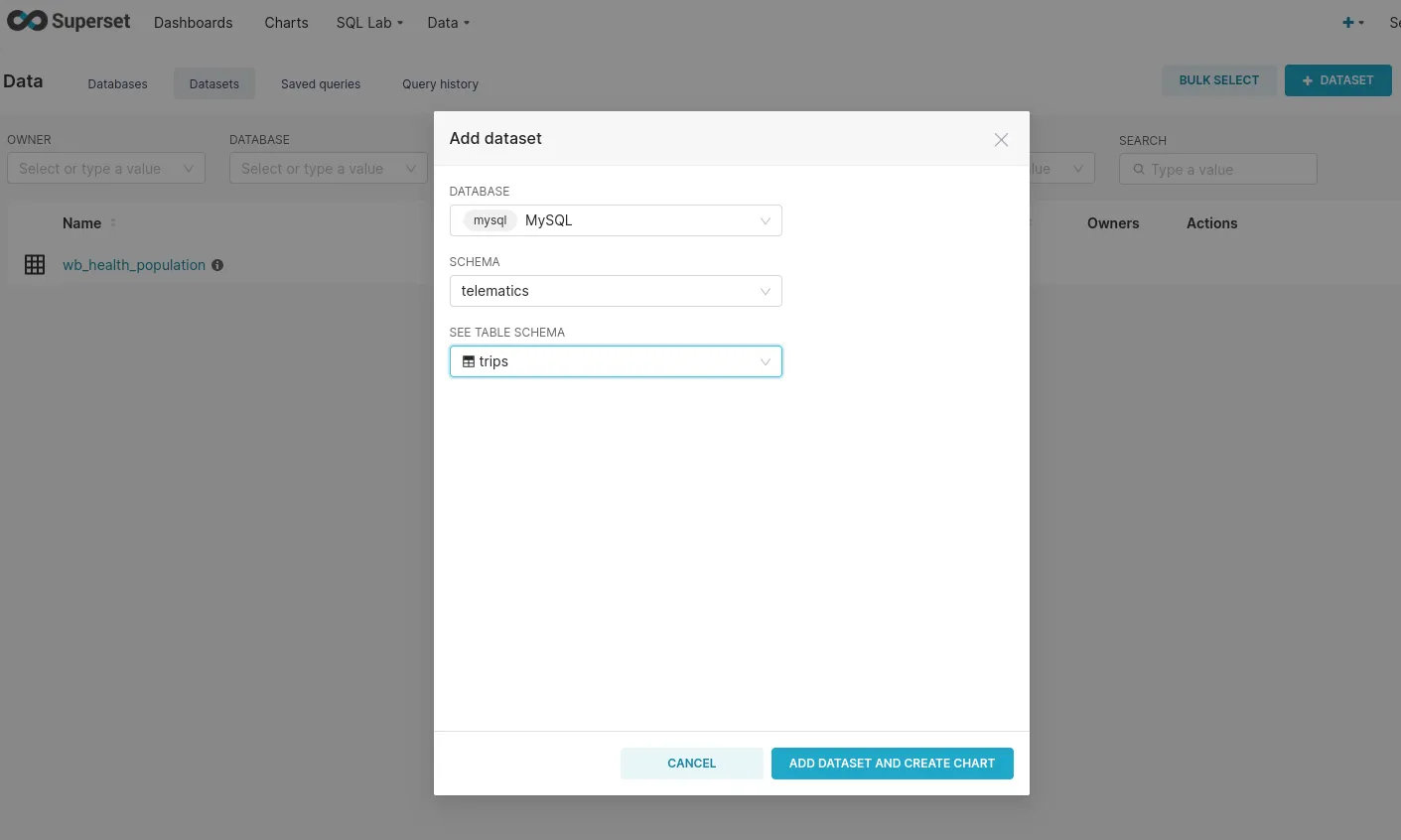
Once it’s running, we can add the trips table as a dataset:

(Keep in mind that, while running in docker, superset will try to use your service account from a different IP than your computer, so GRANT ALL PRIVILEGES ON telematics.* TO 'telematics'@'127.0.01'; or similar does not work!)

Create charts & dashboard

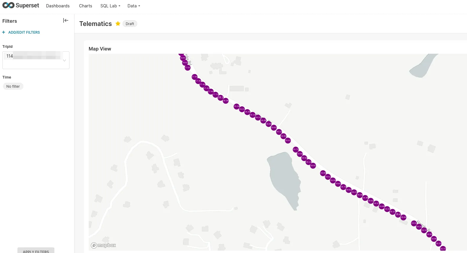
Creating custom charts & a dashboard is also pretty straightforward and my (very basic one) looked like this:

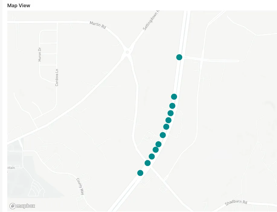
Zooming in on a (synthetic) trip shows individual points:

Note the distance between the points. In this example, the reason for this pattern is simply the way the data has been generated - see below for some thoughts and issues around synthetic testing.

Visualization vs. Analysis

But even with real trips, at a sample rate of 1 sample/s and a speed of 60 miles/hr (or 26.82 meters/s), our measured points would be almost 27 meters or 88 ft apart.

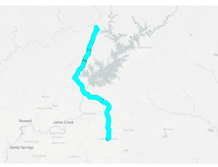
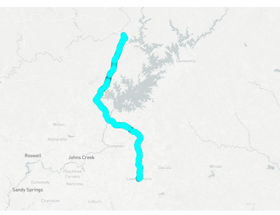
Zoomed out, however, this is a much more coherent trip, even with synthetic data:

The problems with bad sample rates (which can also happen by simply not finding a GPS fix, see “Issues during testing” above!) is that analysis of this data is difficult, even if the zoomed out view (this trip would take about an hour in real life) is certainly coherent.

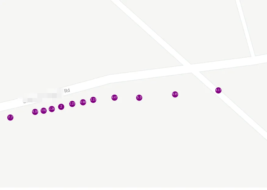
Compare this to the zoomed in view of a real trip collected while driving:

A much more consistent sample rate. However, we can see the GPS precision (or lack thereof) in action once we’re zoomed in real far:

Again, I did not go off-road there. The labels represent speed in meters per second.

However, with this data, we could actually calculate some interesting KPIs via WINDOW functions, such as acceleration or bearing via some trigonometry.

Superset vs `geopandas` + `folium`

This whole process is eons easier than dealing with (the undoubtedly fantastic!) Python libraries like geopandas or folium. Open source data visualization has come a long way over the years, and not having to know what on earth GeoJSON is is surely helpful to make this more accessible.

However, this particular chart type is missing some of the flexibility e.g. folium would give - it’s great at rendering clusters of points, not such my individual points.

However, we can use the deck.gl Geojson map type and get close-ish to what one does with e.g. folium. Since MySQL (and MariaDB) supports spatial functions, we can add a custom column:

1
SELECT ST_AsGeoJSON(POINT(lat,lon)) FROM telematics.trips t 

Yields valid geojson: {"type": "Point", "coordinates": [XXX, YYY]}

Or, why not create an aggregate view?

 1
 2
 3
 4
 5
 6
 7
 8
 9
10
11
12
13
14
15
16
17
18
19
CREATE OR REPLACE VIEW telematics.tripLines AS (
SELECT
	tripId,
	ST_AsGeoJSON(
		LineStringFromText(
			CONCAT("LINESTRING(", 
				GROUP_CONCAT(
				CONCAT(lon, " ", lat))
				, ")")
		) 
	) as tripLine,
	AVG(speed) as averageSpeed,
	COUNT(*) as points,
	MIN(ts) as start_ts,
	MAX(ts) as end_ts
FROM (SELECT * FROM telematics.trips ORDER BY ts ASC) t
GROUP BY
	tripId
)

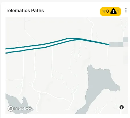
We then can use this data to render smooth lines:

But cracks are starting to show: In order to color these lines in, you need custom JavaScript and for some reason, it did not take my clearly well formated geojson. But it is possible!

Conclusion

This was a lot harder than I thought it would be and hence, was a fantastic learning-by-doing exercise. I’m decently familiar with all the things I’ve used here, but starting from scratch, including setting up all infrastructure down to the Linux image was an experience.

Just, looking at the code, you’d probably say “That doesn’t look that hard!” - and you’d be right. But as I’ve called out above (and am about to again), the devil’s truly in the tiniest of details here.

Things that broke

Things that broke, in no particular order -

armv6 support for Docker
A mini-USB cable
The Raspbian iso file while trying to re-size and chroot into it, repeatedly
My spice grinder (that one was unrelated, but it was unreasonably tedious to repair and I’m shaming it publicly here)
The caching logic with redis
java.io.NotSerializableException: Non-serializable lambda in Flink
systemd and gpsd and of course, the combination thereof
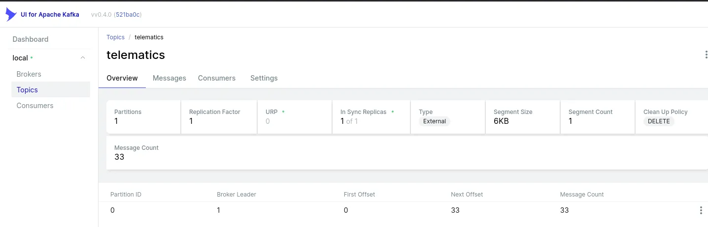
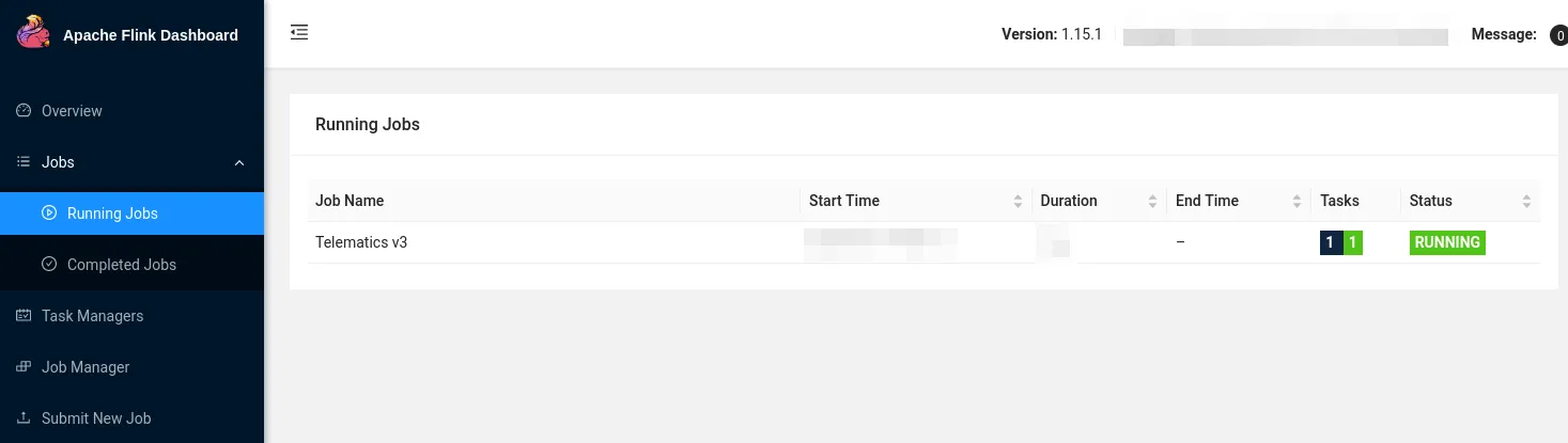
Distributed systems such as Kafka and Flink via Docker as single-node instances - much more pleasant than bare metal installs, but annoying for different reasons, especially once you deploy them alongside things like Kafka UI or Kafka Registry or Kafka Registry UI (things I didn’t even write about here, expect for screenshots)
The Mapbox API key for Apache Superset (it’s an environment variable, who knew?)
udev mappings
The Flink TaskManager randomly crashes and I haven’t even read any logs yet
gpsfake with apparmor and my root access to /dev/pts/
Everything relating to a physical device - see above (I have since purchased a backup device with a different chipset)
Frankly, various other things I probably forgot

Being intentionally offline

Due to all these issues, this was extremely interesting to test. I’ve mentioned synthetic data and integration tests before. We’re probably all used to network and system outages, and that’s why doing something along those lines:

1
2
3
4
5
6
def getGpsRecords(query: Query): IO[List[GpsRecord]] = {
	for {
		data <- queryDatabase(query)
		res = data.filter(r => r.lat != 0f)
	} yield res
}

Is so delightful (it fails fast, predictably, and has a type signature to support it). At the very least, we know to throw an Exception and recover from it eventually or at least fail gracefully and try again later. We can even say queryDatabase(query).handleErrorWith(e => ...), since we know from the type that an Exception is a possibility.

In this case, a lot of what is usually good advice just goes out the window.

Once you’re dealing with a system which intentionally is offline, things change quite a bit. A usual strategy of creating & caching an expensive client (say, Kafka) doesn’t work at all, once you realize that you can’t keep that connection alive, since you expect to be offline any time soon. Testing this at home, of course, works well - every time the application is started or debugged, it can talk to Kafka. If it can’t, you automatically assume you broke something.

Also, due to the nature of GPS, testing has to be in-person and on the road, in real conditions - unit and integration tests can only do so much. A quick trip down the road isn’t hard, per se, but it’s much more effort than running a test suite.

The closest I’ve dealt with something like that in the past was an herein unspecified project that used physical RFID scanners and required frequent trips to the midwest and delightful conversations about grain elevators with Uber drivers while there.

`gpsfake`

“But…!”, I hear you ask. “There’s gpsfake, is there not? Say, does it not open…”

… a pty (pseudo-TTY), launches a gpsd instance that thinks the slave side of the pty is its GNSS device, and repeatedly feeds the contents of one or more test logfiles through the master side to the GNSS receiver.
https://gpsd.gitlab.io/gpsd/gpsfake.html

Why yes, of course there is! But it took me much more time than I’m willing to admit until I realized that this:

 1
 2
 3
 4
 5
 6
 7
 8
 9
10
11
12
13
❯ sudo gpsfake output.nmea -n
/usr/bin/gpsfake:21: DeprecationWarning: The distutils package is deprecated and slated for removal in Python 3.12. Use setuptools or check PEP 632 for potential alternatives
  from distutils import spawn
Processing output.nmea
gpsd:ERROR: SER: device open of /dev/pts/3 failed: Permission denied - retrying read-only
gpsd:ERROR: SER: read-only device open of /dev/pts/3 failed: Permission denied
gpsd:ERROR: SER: device open of /dev/pts/3 failed: Permission denied - retrying read-only
gpsd:ERROR: SER: read-only device open of /dev/pts/3 failed: Permission denied
gpsd:ERROR: /dev/pts/3: device activation failed, freeing device.
gpsfake: log cycle of output.nmea begins.
❯ ll /dev/pts/3
crw-rw-rw- 1 christian tty 136, 3 Aug 25 17:46 /dev/pts/3
# tf?

Was caused by:

1
2
3
4
5
6
7
8
9
newfstatat(AT_FDCWD, "/tmp/gpsfake-39276.sock", {st_mode=S_IFSOCK|0775, st_size=0, ...}, 0) = 0
socket(AF_UNIX, SOCK_STREAM|SOCK_CLOEXEC, 0) = 8
connect(8, {sa_family=AF_UNIX, sun_path="/tmp/gpsfake-39276.sock"}, 25) = 0
sendto(8, "+/dev/pts/10\r\n\0", 15, 0, NULL, 0) = 15
recvfrom(8, gpsd:ERROR: SER: device open of /dev/pts/10 failed: Permission denied - retrying read-only
gpsd:ERROR: SER: read-only device open of /dev/pts/10 failed: Permission denied
"ERROR\n", 12, 0, NULL, NULL) = 6
close(8)                                = 0
wait4(39278, gpsd:ERROR: SER: device open of /dev/pts/10 failed: Permission denied - retrying read-only

Note: “Once you need strace, just stop” is usually a more reasonable approach.

And what can even deny root access to run a stupid syscall like sendto(2)? Correct, apparmor and SELinux. (╯°□°)╯︵ ┻━┻

1
2
3
4
5
6
❯ sudo apparmor_status
apparmor module is loaded.
29 profiles are loaded.
27 profiles are in enforce mode.
   ...
   /usr/sbin/gpsd

This was one of those things where there’s one mailing list thread from 2012 as a response that doesn’t solve the issue.

> Regressions run just fine here.

Does me no good. :-)

For the record, if you’re here via Google: Just set /usr/sbin/gpsd to complain mode and it’ll work…

Anyways - this is synthetic data. It does not test getting an actual GPS fix in the car, the service starting alongside the vehicle, gpsd talking to the right device, changing WiFi environments, intentional and unintentional network outages, weather conditions, tree canopy and so on and so forth.

You’ve seen some of this data in the previous section - it doesn’t have realistic speeds, altitudes, pauses, traffic conditions etc.

It also, very obviously, did not catch the hardware / configuration issue we’ve dealt with a handful of paragraphs above. Needless to say, it wouldn’t have caught the duplicate record issue neither.

TBD - move

Next Steps?

While this was fun (and very usable! Tried it in 2 cars, even!), we really should really be able to…

Write Apache Iceberg instead of plain SQL
Make it actually exactly-once
Generally, do more logic and aggregation in the Flink stream - right now, it’s just a dumb sink
Automatically power the Raspberry on and off (not just the application). This currently happens because my truck cuts USB power after a while, not because it shuts itself down - works in my vehicle, but probably not in yours.
Integrate OBD2 data
Identify trips more consistently
Improve the domain model. It could be much richer
Maybe customize some visualization
Fix some gpsd mishaps and dig deeper and avoid the stupid workarounds

How this looked from the outside. [Credit: Author]

So long and thanks for all the fish

Anyways - I hope you enjoyed it. If you want to try this for yourself, all code is on GitHub as usual.

All development and benchmarking was done under GNU/Linux [PopOS! 22.04 on Kernel 5.18] with 12 Intel i7-9750H vCores @ 4.5Ghz and 32GB RAM on a 2019 System76 Gazelle Laptop, using scala 2.12.16

Christian Hollinger